API
Import SpatialDM as:
import spatialdm as sdm
Functions
- spatialdm.stats.rbfweight(X_loc, l=None, cutoff=0.1, n_neighbors=None, n_neighbor_layers=6, single_cell=False, eff_dist=None)
Compute weight matrix based on radial basis function. cutoff & n_neighbors are two alternative options to restrict signaling range.
- Parameters:
l – radial basis function parameter, need to be customized for optimal weight gradient and to restrain the range of signaling before downstream processing.
cutoff – (for secreted signaling) minimum weight to be kept from the rbf weight matrix. Weight below cutoff will be made zero
n_neighbors – (for secreted signaling) number of neighbors per spot from the rbf weight matrix.
n_neighbor_layers – (for adjacent signaling) number of neighbor layers per spot from the rbf weight matrix. Non-neighbors will be made 0
single_cell – if single_cell, diagonal will be made 0.
eff_dist – the alternative way to set l parameter by restricting the effective distance.
- Returns:
secreted signaling weight matrix: W_spatial, and adjacent signaling weight matrix: KNN_connectivities
Examples
>>> import numpy as np
>>> from spatialdm.stats import rbfweight
>>> X_loc = np.vstack([np.repeat(range(10), 10), np.tile(range(10), 10)]).T
>>> spatial_W, KNN_connect = rbfweight(X_loc, l=1.2, n_neighbors=16)
>>> import matplotlib.pyplot as plt
>>> plt.scatter(X_loc[:, 0], X_loc[:, 1], c=spatial_W.toarray()[35], s=100)
>>> plt.show()
(
Source code,png)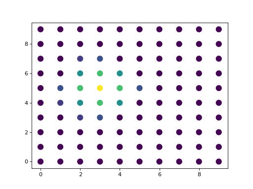
- spatialdm.stats.Moran_R(X, Y, spatial_W, standardise=True, nproc=1)
Computing Moran’s R for pairs of variables
- Parameters:
X – Variable 1, (n_sample, n_variables) or (n_sample, )
Y – Variable 2, (n_sample, n_variables) or (n_sample, )
spatial_W – spatial weight matrix, sparse or dense, (n_sample, n_sample)
nproc – default to 1. Numpy may use more without much speedup.
- Returns:
(Moran’s R, z score and p values)
Examples
>>> import numpy as np
>>> from spatialdm.stats import rbfweight, Moran_R
>>> np.random.seed(0)
>>> X1 = np.random.rand(100, 5)
>>> X2 = np.random.rand(100, 5)
>>> X2[:-1, 0], X2[:, 1], X2[1:, 2] = X1[1:, 0], X1[:, 1], X1[:-1, 2]
>>> X2 = X2 + 0.01 * np.random.rand(100, 5)
>>> X_loc = np.vstack([np.repeat(range(10), 10), np.tile(range(10), 10)]).T
>>> spatial_W, KNN_connect = rbfweight(X_loc, l=1.2, n_neighbors=16)
>>> R, z, p = Moran_R(X1, X2, spatial_W)
>>> print(R, z, p)
>>> import matplotlib.pyplot as plt
>>> fig = plt.figure(figsize=(6, 3))
>>> plt.subplot(1, 2, 1)
>>> plt.scatter(X_loc[:, 0], X_loc[:, 1], c=X1[:, 0], s=100)
>>> plt.subplot(1, 2, 2)
>>> plt.scatter(X_loc[:, 0], X_loc[:, 1], c=X2[:, 0], s=100)
>>> plt.tight_layout()
>>> plt.show()
(
Source code,png)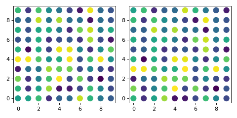
Datasets
The spatialdm.datasets module provides functions for loading and accessing spatial transcriptomics datasets. The following datasets are currently available:
dataset.melanoma(): Sample 1 rep 2 human melanoma slide from Thrane’s melanoma dataset.
dataset.SVZ(): Mouse sub-ventricular zone (SVZ) from Eng’s seqfish+ dataset.
dataset.A1(): Adult colon with colorectal cancer or IBD, pcw: Adult.
dataset.A2(): Adult colon with colorectal cancer or IBD, pcw: Adult.
dataset.A3(): Fetal colon, pcw: 12PCW.
dataset.A4(): Fetal colon, pcw: 19PCW.
dataset.A6(): Fetal small intestine, pcw: 12PCW.
dataset.A7(): Fetal small intestine, pcw: 12PCW.
dataset.A8(): Fetal small intestine, pcw: 12PCW.
dataset.A9(): Fetal small intestine, pcw: 12PCW.
Usage
To use the spatialdm.datasets module, simply import it as follows:
from spatialdm.datasets import dataset
Then, you can load a dataset using the corresponding function. For example, to load the melanoma dataset:
adata = dataset.melanoma()
This will return an anndata object containing the expression data for the melanoma dataset in .X, the cell type decomposition values in .obs, and the spatial coordinates in .obsm[‘spatial’].