SpatialDM tutorial with melanoma data
You may also run it on Google Colab with this link: melanoma.ipynb
TO run it on Google Colab (or a new environment), please change this section into code (or copy into a new code block) for installing the following packages. Note, please only install the package if you need (required on colab). For your local environment, you only need to install them for the first time.
# optionally use an older version of scipy (also works till v1.15.3)
!pip install scipy==1.11.4

# install anndata <= 0.10.8 to avoid complicated cupy package
!pip install anndata==0.10.8

# install latest SpatialDM from github directly
!pip install -U git+https://github.com/StatBiomed/SpatialDM

!pip install SparseAEH
[1]:
import os
import pandas as pd
import numpy as np
import anndata as ann

import spatialdm as sdm
from spatialdm.datasets import dataset
import spatialdm.plottings as pl

import matplotlib.pyplot as plt
print("SpatailDM version: %s" %sdm.__version__)
SpatailDM version: 0.3.0
[ ]:
The melanoma dataset from Thrane, et al. 2018 Caner Cell was publicly available. We obtained raw counts, pre-processed log counts, and spatial coordinates from Matt Stone (Git repository). For easier reuse, we included them in an anndata object which can be loaded directly in SpatialDM Python package.
We can see the histology image below from the orignal supplementary figure (the first sample):

For the cell type annotation, we can visualize it from SpatialDM’s paper Figure 2b.
[2]:
adata = dataset.melanoma()
adata.X,adata.raw,adata.obs,adata.obsm['spatial']Step 0: SpatialDM object and preprocessing
We generate a suitable weight matrix for the SpatialDM object at first. Here considering the scale of the spatial coordinates and spot-spot distance (200 micrometers here), we set radial basis kernel parameter l = 1.2, and trimmed all weights < 0.2 (cutoff) to match the normal range of CCC (200 micrometers, 1 spot away from the sender cell here)
Note Alternative to the cutoff parameter, we can set n_neighbors to around 8 to restrain the range of CCC.
[3]:
# weight_matrix by rbf kernel
sdm.weight_matrix(adata, l=1.2, cutoff=0.2, single_cell=False)
Note
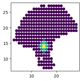
If the scale of the spatial coordinates is larger (e.g. several thousand in the intestinal example) or smaller, or when the spot-spot distance varies (which is common for different platforms), the l can be very different. It’s a crucial step to determine a suitable l to match the biological context. We recommend the following plotting to check the resulting weight matrix from the previous step. If needed, users can run weight_matrix iteratively to decide the most optimal l and
cutoff. You can also use the parameter eff_dist to help you determine l. It stands for the maximum distance between two points that can influence each other. eff_dist also relies heavily on the scale of the spatial coordinates. Try to provide at least one good estimate of l and eff_dist to enable the clustering algorithm function better.
[4]:
# visualize range of interaction
import matplotlib.pyplot as plt
plt.figure(figsize=(3,3))

plt.scatter(adata.obsm['spatial'][:,0], adata.obsm['spatial'][:,1],
            c=adata.obsp['weight'].toarray()[50])
plt.show()
Next step is to extract valid LR pairs from the database (by default, we use CellChatDB). Filtering out sparsely expressed ligand or receptor (e.g. 3) can help us get more interpretable results later.
[5]:
# find overlapping LRs from CellChatDB
sdm.extract_lr(adata, 'human', min_cell=3)
Step 1.1: Global selection of spatially co-expressed LR pairs (z-score approach)
It is a crucial step to identify dataset-specific interacting LR pairs (global selection) for ensuring quality analysis and reliable interpretation of the putative CCC. With high computation efficiency, SpatialDM can complete global selection in seconds.
[6]:
import time
start = time.time()

# global Moran selection
sdm.spatialdm_global(adata, method='z-score', nproc=1)

# select significant pairs
sdm.sig_pairs(adata, method='z-score', fdr=True, threshold=0.1)

print("%.3f seconds" %(time.time()-start))
10.597 seconds
We used fdr corrected global p-values and a threshold FDR < 0.1 (default) to determine which pairs to be included in the following local identification steps. There are 103 pairs being selected in this data.
[7]:
print(adata.uns['global_res'].selected.sum())
adata.uns['global_res'].sort_values(by='fdr').head()
172
[7]:
| Ligand0 | Ligand1 | Ligand2 | Receptor0 | Receptor1 | Receptor2 | z_pval | z | fdr | selected | |
|---|---|---|---|---|---|---|---|---|---|---|
| CCL21_CCR7 | CCL21 | None | None | CCR7 | None | None | 2.351186e-63 | 16.761051 | 2.118419e-60 | True |
| CD99_CD99 | CD99 | None | None | CD99 | None | None | 1.786933e-60 | 16.361968 | 8.050133e-58 | True |
| PECAM1_PECAM1 | PECAM1 | None | None | PECAM1 | None | None | 6.034266e-50 | 14.813025 | 1.812291e-47 | True |
| ESAM_ESAM | ESAM | None | None | ESAM | None | None | 6.911664e-48 | 14.490942 | 1.556852e-45 | True |
| SPP1_ITGAV_ITGB5 | SPP1 | None | None | ITGAV | ITGB5 | None | 2.987723e-46 | 14.229915 | 5.383876e-44 | True |
[ ]:
Step 1.2: Local selection of interacting spots (z-score approach)
Local selection is then carried out for the selected 103 pairs to identify where the LRI take place, in a single-spot resolution.
[8]:
start = time.time()
# local spot selection
sdm.spatialdm_local(adata, method='z-score', nproc=1)

# significant local spots
sdm.sig_spots(adata, method='z-score', fdr=False, threshold=0.1)

print("%.3f seconds" %(time.time()-start))
1.548 seconds
By default, local selection is performed for all selected pairs in the previous step.
Note
Apply an array of integer indices of selected pairs to select_num to run local selection in selected pairs
The global and local results are easily accessible through global_res and local_perm_p or local_z_p
Step 1.3 (exploratory): Visualize pair(s)
SpatialDM provides plotting utilities for general summary of global results:
[9]:
pl.global_plot(adata, pairs=['SPP1_CD44', 'CSF1_CSF1R', 'VEGFA_VEGFR2', 'ANGPTL4_SDC2'],
               figsize=(6,5), cmap='RdGy_r', vmin=-1.5, vmax=2)
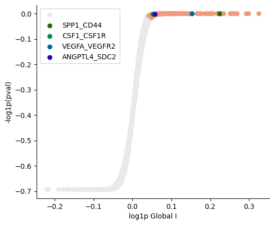
Known melanoma-related pairs were all observed in the selected pairs. It would then be meaningful to investigate the spatial context of their interactions.
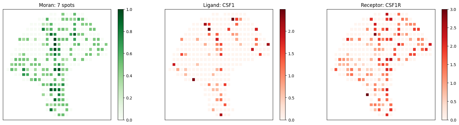
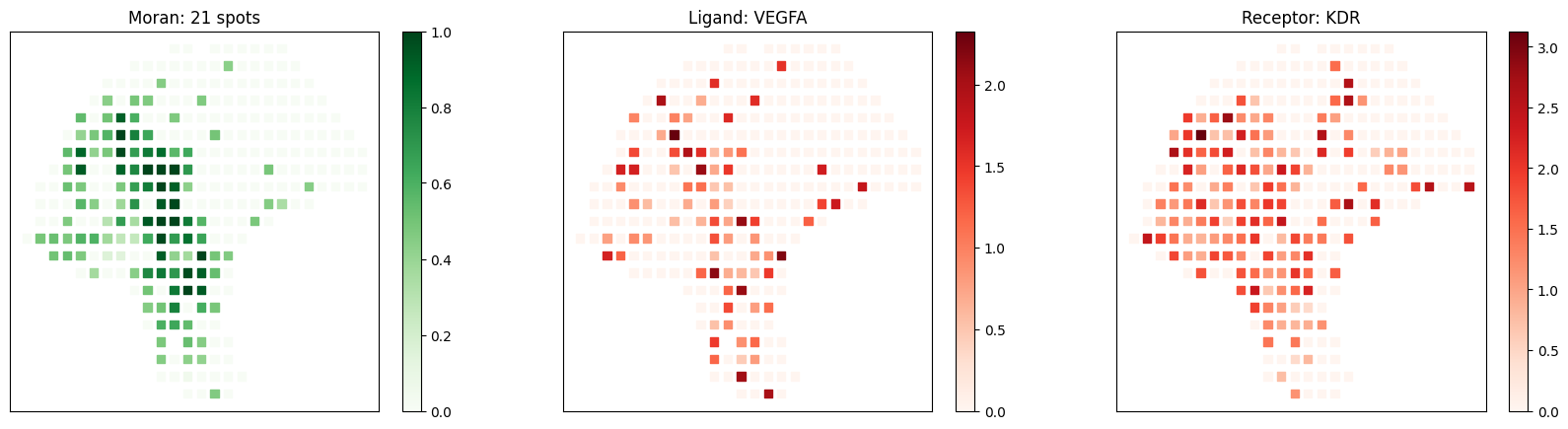
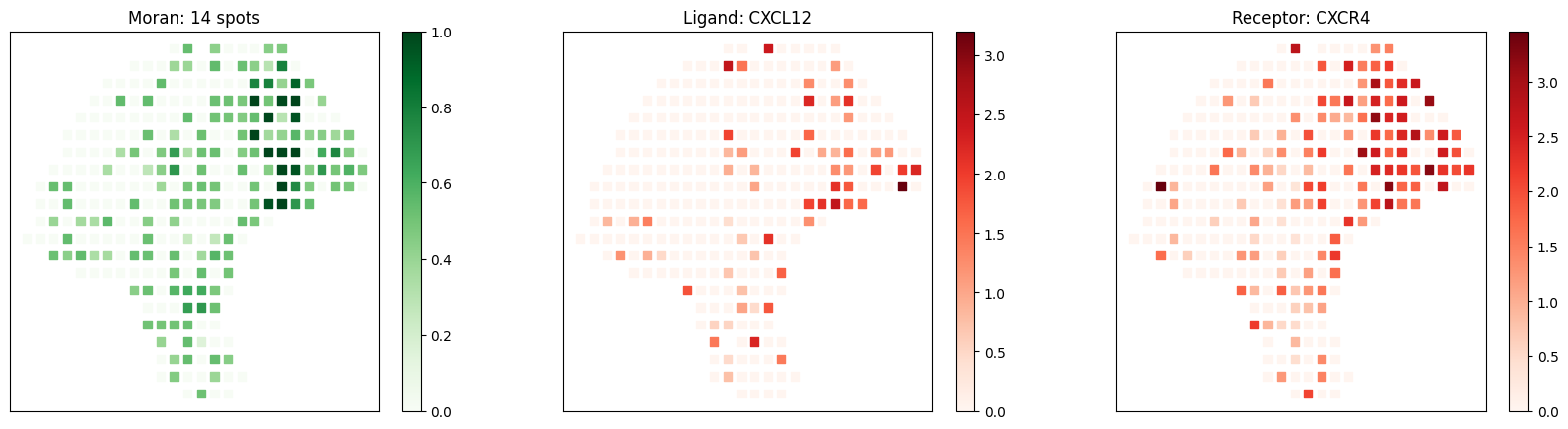
[10]:
# visualize known melanoma pairs
pl.plot_pairs(adata, ['CSF1_CSF1R', 'VEGFA_VEGFR2', 'CXCL12_CXCR4'], marker='s')
[ ]:
Step 2: Spatial Clustering of Local Spots
SparseAEH allows clustering of spatially auto-correlated genes. Here, we repurposed SpatialDE to identify spatially auto-correlated interactions by using binary local selection status as input.
[11]:
from SparseAEH import MixedGaussian
from SparseAEH.plot import plot_clusters
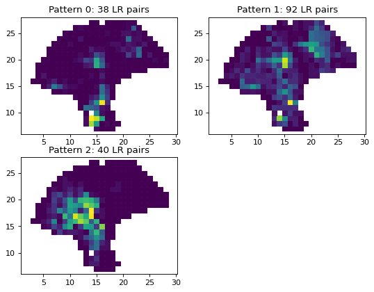
Filter out sparse interactions with fewer than 3 identified interacting spots. Cluster into 6 patterns.
[12]:
lr_idx = adata.uns['local_stat']['n_spots'] > 2
bin_spots = adata.uns['selected_spots'].astype(int)[lr_idx]
Y = bin_spots.to_numpy()

print(bin_spots.shape[0], "pairs used for spatial clustering")
170 pairs used for spatial clustering
[13]:
gaussian = MixedGaussian(adata.obsm['spatial'], group_size=16, d=30, l=1e-5)
cluster = gaussian.run_cluster(Y.T, 3, iter=50, init_mean='k_means')
Iteration 0
updating variance
Iteration 1
[ ]:
[14]:
def plot_clusters(gaussian, label='counts', s=15):
    k = gaussian.K
    h = np.ceil(np.sqrt(k)).astype(int)
    w = np.ceil(k/h).astype(int)
    for i in range(gaussian.K):
        plt.subplot(h, w, i + 1)
        plt.scatter(gaussian.kernel.spatial[:, 0],
                    gaussian.kernel.spatial[:, 1],
                    marker = 's', c=gaussian.mean[:, i],
                    cmap="viridis", s=s)
        plt.axis('equal')
        # plt.gca().invert_yaxis()
        if label == 'counts':
            plt.title('Pattern %d: %d LR pairs'
                      %(i, np.sum(gaussian.labels == i)))
        else:
            plt.title('Pattern %d: %.3f proportion' %(i, gaussian.pi[i]))
[15]:
plt.figure(figsize = (8, 6), dpi=80)
plot_clusters(gaussian, s=38)
plt.show()
[ ]:
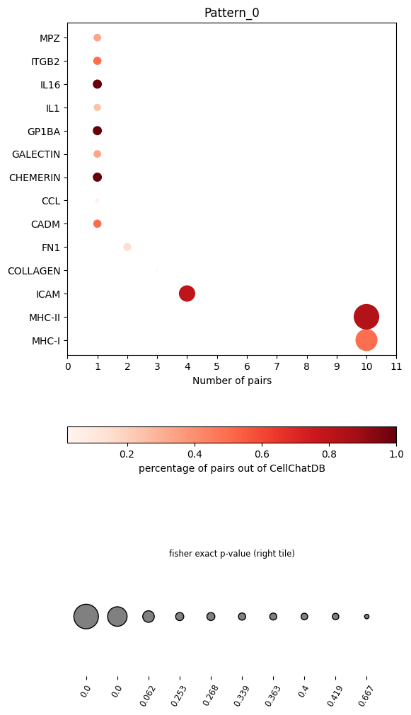
Step 3: Pathway enrichment of spatial clusters of LR pairs
SpatialDM provides compute_pathway function to group a list of interactions based on the pathways they belong. The input can be a dictionary of several lists.
[16]:
dic=dict()
for i in range(gaussian.K):
    dic['Pattern_{}'.format(i)]=bin_spots.index[gaussian.labels==i]
Save the anndata file to retrieve later
[17]:
adata_out = adata.copy()
adata_out.uns['local_stat']['local_permI'] = 'None'
adata_out.uns['local_stat']['local_permI_R'] = 'None'

# sdm.write_spatialdm_h5ad(adata_out, filename='mel_sdm_out.h5ad')
# sdm.read_spatialdm_h5ad(filename='mel_sdm_out.h5ad')
Conduct pathway enrichment analysis
[18]:
pathway_res = sdm.compute_pathway(adata,dic=dic)
pathway_res
[18]:
| total_genes | query_genes | overlapped_genes | background_mapped_genes | background_unmapped_genes | selected | fisher_p | pattern | |
|---|---|---|---|---|---|---|---|---|
| pathway | ||||||||
| ACTIVIN | INHBA_ACVR1B_ACVR2A INHBA_ACVR1B_ACVR2A... | {HLA-DMB_CD4, HLA-DRB5_CD4, CCL5_CCR1, HLA-C_C... | {} | {} | {ANGPTL4_SDC4, TNC_ITGAV_ITGB3, C3_ITGAM_ITGB2... | 0 | 1.0 | Pattern_0 |
| ADIPONECTIN | ADIPOQ_ADIPOR1 ADIPOQ_ADIPOR1 ADIPOQ_ADIPOR... | {HLA-DMB_CD4, HLA-DRB5_CD4, CCL5_CCR1, HLA-C_C... | {} | {} | {ANGPTL4_SDC4, TNC_ITGAV_ITGB3, C3_ITGAM_ITGB2... | 0 | 1.0 | Pattern_0 |
| AGRN | AGRN_DAG1 AGRN_DAG1 Name: interaction_name,... | {HLA-DMB_CD4, HLA-DRB5_CD4, CCL5_CCR1, HLA-C_C... | {} | {} | {ANGPTL4_SDC4, TNC_ITGAV_ITGB3, C3_ITGAM_ITGB2... | 0 | 1.0 | Pattern_0 |
| ALCAM | ALCAM_CD6 ALCAM_CD6 Name: interaction_name,... | {HLA-DMB_CD4, HLA-DRB5_CD4, CCL5_CCR1, HLA-C_C... | {} | {} | {ANGPTL4_SDC4, TNC_ITGAV_ITGB3, C3_ITGAM_ITGB2... | 0 | 1.0 | Pattern_0 |
| AMH | AMH_AMHR2_BMPR1A AMH_AMHR2_BMPR1A AMH_AMHR2... | {HLA-DMB_CD4, HLA-DRB5_CD4, CCL5_CCR1, HLA-C_C... | {} | {} | {ANGPTL4_SDC4, TNC_ITGAV_ITGB3, C3_ITGAM_ITGB2... | 0 | 1.0 | Pattern_0 |
| ... | ... | ... | ... | ... | ... | ... | ... | ... |
| VISFATIN | NAMPT_INSR NAMPT_INSR NAMPT_I... | {COL9A3_ITGA2_ITGB1, OCLN_OCLN, ANGPTL4_SDC4, ... | {} | {} | {HLA-DRB5_CD4, C3_ITGAM_ITGB2, CCL21_CCR7, SEL... | 0 | 1.0 | Pattern_2 |
| VWF | VWF_ITGAV_ITGB3 VWF_ITGAV_I... | {COL9A3_ITGA2_ITGB1, OCLN_OCLN, ANGPTL4_SDC4, ... | {} | {VWF_GP1BA_GP1BB_GP5_GP9} | {HLA-DRB5_CD4, C3_ITGAM_ITGB2, CCL21_CCR7, SEL... | 0 | 1.0 | Pattern_2 |
| WNT | WNT10A_FZD9_LRP6 WNT10A_FZD9_LRP6 WNT10A_... | {COL9A3_ITGA2_ITGB1, OCLN_OCLN, ANGPTL4_SDC4, ... | {} | {} | {HLA-DRB5_CD4, C3_ITGAM_ITGB2, CCL21_CCR7, SEL... | 0 | 1.0 | Pattern_2 |
| XCR | XCL1_XCR1 XCL1_XCR1 Name: interaction_name,... | {COL9A3_ITGA2_ITGB1, OCLN_OCLN, ANGPTL4_SDC4, ... | {} | {} | {HLA-DRB5_CD4, C3_ITGAM_ITGB2, CCL21_CCR7, SEL... | 0 | 1.0 | Pattern_2 |
| ncWNT | WNT5B_FZD9 WNT5B_FZD9 WNT5B_FZD8 WNT5B_F... | {COL9A3_ITGA2_ITGB1, OCLN_OCLN, ANGPTL4_SDC4, ... | {} | {} | {HLA-DRB5_CD4, C3_ITGAM_ITGB2, CCL21_CCR7, SEL... | 0 | 1.0 | Pattern_2 |
408 rows × 8 columns
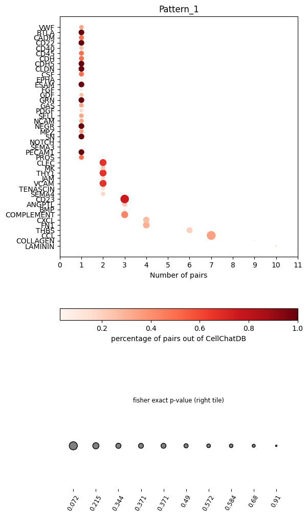
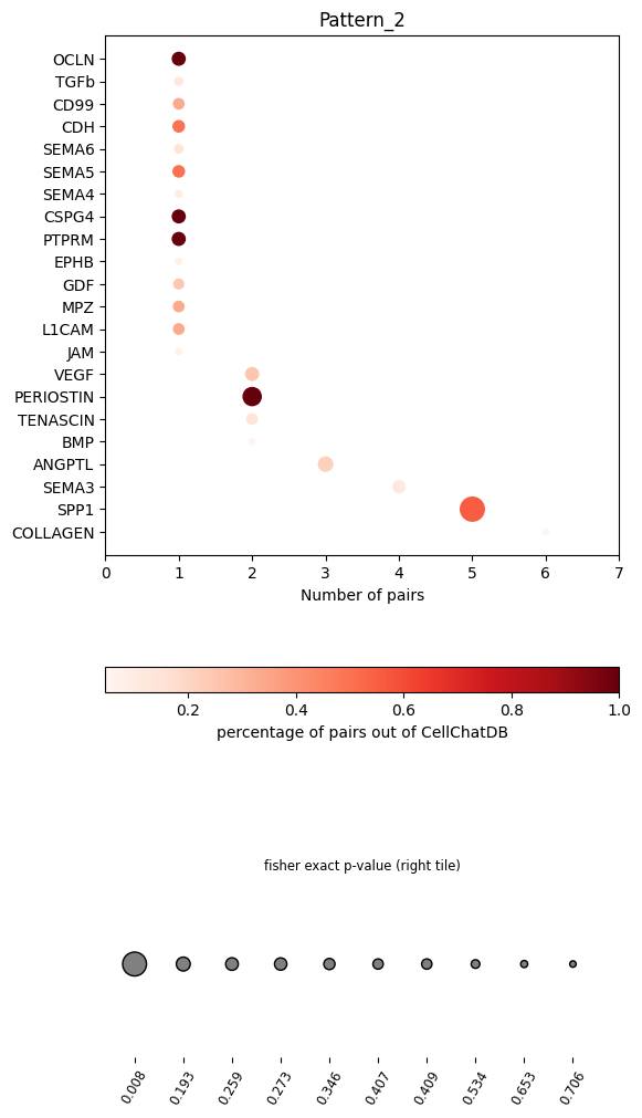
In the dot plot of the lymphoid-associated pattern, we identified CD23 and other immune-related pathways.
[19]:
pl.dot_path(pathway_res, figsize=(6,12))
[ ]:
Misc:
SpatialDM provides chord_celltype and other chord diagrams to visualize the aggregated cell types (or interactions).
Change the next block from text to code to make the chord plot:
adata.obsm['celltypes'] = adata.obs[adata.obs.columns] pl.chord_celltype(adata, pairs=['FCER2A_CR2'], ncol=1, min_quantile=0.01) # save='mel_FCER2A_CR2_ct.svg'[ ]: