Differential analyses (z-score approach)
[1]:
import os
import pandas as pd
import numpy as np
import anndata as ann
import spatialdm as sdm
from spatialdm.datasets import dataset
import spatialdm.plottings as pl
print("SpatailDM version: %s" %sdm.__version__)


SpatailDM version: 0.0.7
z-score selection in batch
[2]:
data=["A1","A2","A3","A4","A6","A7","A8","A9"]
The intestine dataset from Corbett, et al. was publicly available on STAR-FINDer, from which we obtained raw counts and spatial coordinates, and log-transformed to normalize on the spot-level. Rawcounts (.raw), logcounts (.X), cell types (.obs), and spatial coordinates (.obsm['spatial']) have been included in the corresponding anndata object which can be loaded directly in SpatialDM Python package.
[4]:
A1 = dataset.A1()
A2 = dataset.A2()
A3 = dataset.A3()
A4 = dataset.A4()
A6 = dataset.A6()
A7 = dataset.A7()
A8 = dataset.A8()
A9 = dataset.A9()
Note
[5]:
samples = [A1,A2,A3,A4,A6,A7,A8,A9]
Considering the scale of the spatial coordinates and spot-spot distance of 100 micrometers, l will be set to 75 here. The parameters here should be determined to match the context of CCC.
[9]:
for adata in samples:
adata.obsm['spatial'] = adata.obsm['spatial'].values
sdm.weight_matrix(adata, l=75, cutoff=0.2, single_cell=False) # weight_matrix by rbf kernel
sdm.extract_lr(adata, 'human', min_cell=3) # find overlapping LRs from CellChatDB
sdm.spatialdm_global(adata, 1000, specified_ind=None, method='z-score', nproc=1) # global Moran selection
sdm.sig_pairs(adata, method='z-score', fdr=True, threshold=0.1) # select significant pairs
sdm.spatialdm_local(adata, n_perm=1000, method='z-score', specified_ind=None, nproc=1) # local spot selection
sdm.sig_spots(adata, method='z-score', fdr=False, threshold=0.1)
print(' done!')
/home/yoyo/miniconda2/envs/CC/lib/python3.9/site-packages/sklearn/utils/validation.py:70: FutureWarning: Pass n_neighbors=6 as keyword args. From version 1.0 (renaming of 0.25) passing these as positional arguments will result in an error
warnings.warn(f"Pass {args_msg} as keyword args. From version "
100%|██████████| 1000/1000 [09:45<00:00, 1.71it/s]
/home/yoyo/miniconda2/envs/CC/lib/python3.9/site-packages/spatialdm/utils.py:130: RuntimeWarning: invalid value encountered in true_divide
X = X/X.max()
100%|██████████| 1000/1000 [00:14<00:00, 69.16it/s]
100%|██████████| 1000/1000 [00:06<00:00, 162.48it/s]
done!
filtered non-expressed LR pairs.
Save selection results in batch
differential test on 6 colon samples (adult vs. fetus)
[10]:
from spatialdm.diff_utils import *
First step is to concatenate all selection results, resulting in a p_df storing p-values across each sample before fdr correction, a tf_df indicating whether each pair is selected in each sample, and a zscore_df which stores z-scores. These will be essential for the differential analyses later.
[11]:
concat=concat_obj(samples, data, 'human', 'z-score', fdr=False)
/home/yoyo/miniconda2/envs/CC/lib/python3.9/site-packages/anndata/_core/anndata.py:1828: UserWarning: Observation names are not unique. To make them unique, call `.obs_names_make_unique`.
utils.warn_names_duplicates("obs")
[12]:
concat.uns['p_df'].head()
[12]:
| A1 | A2 | A3 | A4 | A6 | A7 | A8 | A9 | |
|---|---|---|---|---|---|---|---|---|
| VSIR_IGSF11 | 0.425453 | 0.395138 | 0.598898 | 0.315757 | 0.599201 | 0.327638 | 0.666588 | 0.760361 |
| EFNA5_EPHA7 | 0.510958 | 0.774411 | 0.096287 | 0.039663 | 0.003395 | 0.006287 | 0.058307 | 0.411695 |
| EFNA5_EPHB2 | 0.306913 | 0.104032 | 0.111116 | 0.000113 | 0.079636 | 0.026080 | 0.766981 | 0.515436 |
| EFNB1_EPHA4 | 0.270509 | 0.002146 | 0.019308 | 0.008792 | 0.002633 | 0.008091 | 0.357686 | 0.182043 |
| EFNB1_EPHB2 | 0.428187 | 0.218473 | 0.994771 | 0.010403 | 0.005470 | 0.001725 | 0.217220 | 0.498809 |
[13]:
concat.uns['tf_df'].head()
[13]:
| A1 | A2 | A3 | A4 | A6 | A7 | A8 | A9 | |
|---|---|---|---|---|---|---|---|---|
| VSIR_IGSF11 | False | False | False | False | False | False | False | False |
| EFNA5_EPHA7 | False | False | False | True | True | True | False | False |
| EFNA5_EPHB2 | False | False | False | True | False | True | False | False |
| EFNB1_EPHA4 | False | True | True | True | True | True | False | False |
| EFNB1_EPHB2 | False | False | False | True | True | True | False | False |
[14]:
concat.uns['zscore_df'].head()
[14]:
| A1 | A2 | A3 | A4 | A6 | A7 | A8 | A9 | |
|---|---|---|---|---|---|---|---|---|
| VSIR_IGSF11 | 0.187962 | 0.265951 | -0.250496 | 0.479598 | -0.251280 | 0.446444 | -0.430511 | -0.707466 |
| EFNA5_EPHA7 | -0.027471 | -0.753451 | 1.303003 | 1.754614 | 2.707015 | 2.495596 | 1.569141 | 0.223187 |
| EFNA5_EPHB2 | 0.504619 | 1.258905 | 1.220614 | 3.688469 | 1.407522 | 1.941812 | -0.728942 | -0.038703 |
| EFNB1_EPHA4 | 0.611274 | 2.855859 | 2.068248 | 2.374266 | 2.790333 | 2.404807 | 0.364652 | 0.907606 |
| EFNB1_EPHB2 | 0.180993 | 0.777361 | -2.560322 | 2.311493 | 2.544579 | 2.924481 | 0.781615 | 0.002986 |
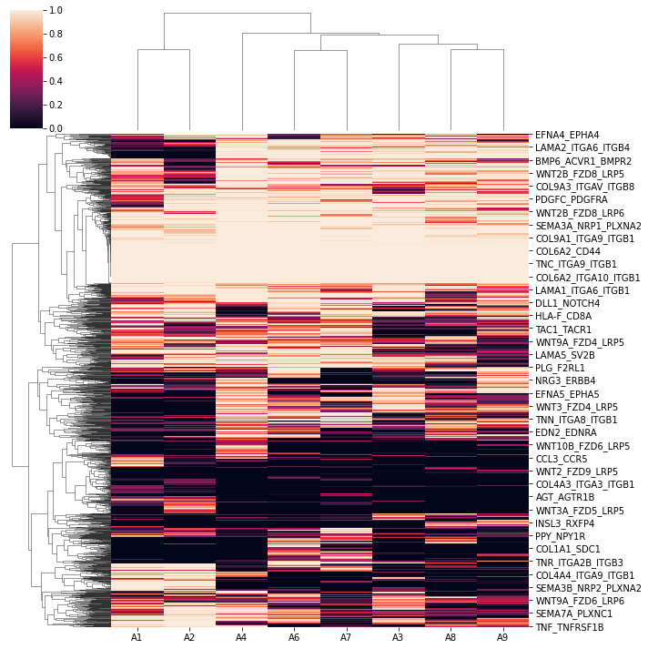
Whole-interactome clustering revealed the dendrogram relationships that are close to the sample kinship
[15]:
import seaborn as sns
sns.clustermap(1-concat.uns['p_df'])
/home/yoyo/miniconda2/envs/CC/lib/python3.9/site-packages/seaborn/matrix.py:649: UserWarning: Clustering large matrix with scipy. Installing `fastcluster` may give better performance.
warnings.warn(msg)
[15]:
<seaborn.matrix.ClusterGrid at 0x7f9c2b7df8e0>
Next, we subset the 6 colon samples (2 adult vs. 4 fetus for differential analyses.
Use 1 and 0 to label different conditions.
Note z-score differential testing will also support differential test among 3 or more conditions, provided with sufficient samples.
[16]:
conditions = np.hstack((np.repeat([1],2), np.repeat([0],4)))
subset = ['A1', 'A2', 'A3', 'A4', 'A8', 'A9']
By differential_test, likelihood ratio test will be performed, and the differential p-values are stored in uns['p_val'], corresponding fdr values in uns['diff_fdr'], and difference in average zscores in uns['diff'].
[17]:
differential_test(concat, subset, conditions)
/home/yoyo/miniconda2/envs/CC/lib/python3.9/site-packages/statsmodels/regression/linear_model.py:903: RuntimeWarning: divide by zero encountered in log
llf = -nobs2*np.log(2*np.pi) - nobs2*np.log(ssr / nobs) - nobs2
/home/yoyo/miniconda2/envs/CC/lib/python3.9/site-packages/spatialdm/diff_utils.py:109: RuntimeWarning: invalid value encountered in double_scalars
LR_statistic[i] = -2 * (reduced_ll - full_ll)
Later, we can focus on differential pairs within 2 contrasting conditions. By default, pairs with z-score difference greater than 30% quantile and a corrected differential significance (.diff_fdr) smaller than 0.1 are selected, while different parameters can be applied in diff_quantile1, diff_quantile2, and fdr_co, respectively.
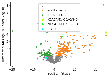
differential_volcano allows easy check for target pair(s) in whether they are differential among conditions and in which condition it’s specific.
[18]:
group_differential_pairs(concat, 'adult', 'fetus')
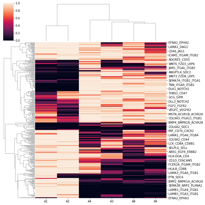
[19]:
pl.differential_dendrogram(concat)
[19]:
<seaborn.matrix.ClusterGrid at 0x7f9871e74f10>
[20]:
pl.differential_volcano(concat, legend=['adult specific', 'fetus specific'])
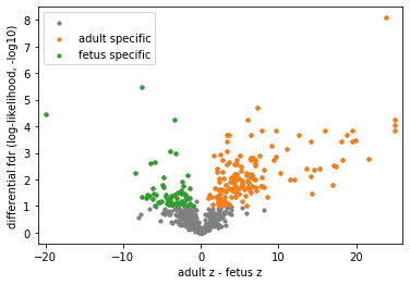
Note
CEACAM1_CEACAM5 is sparsely identified in A3 in addition to two adult slices, but still considered adult-specific by differential analyses. NRG4 was found in human breast milk, and its oral supplementation can protect against inflammation in the intestine. PLG_F2RL1 is sparsely and exclusively identified in fetal samples with consistent cell type enrichment. Please refer to our manuscript for more discussions.
[27]:
pl.differential_volcano(concat, pairs=['CEACAM1_CEACAM5', 'NRG4_ERBB2_ERBB4', 'PLG_F2RL1'],
legend=['adult specific', 'fetus specific'], )
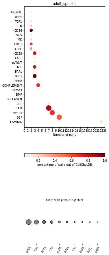
[25]:
pl.dot_path(concat, 'adult_specific', cut_off=2, figsize=(5,15))
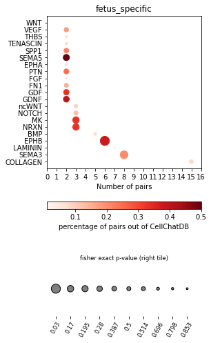
[26]:
pl.dot_path(concat, 'fetus_specific', cut_off=2, figsize=(4,8))
[37]:
A1.uns['geneInter'].loc[(A1.uns['geneInter'].pathway_name=='EGF') \
&(A1.uns['geneInter'].index.isin(A1.uns['selected_spots'].index))]
[37]:
| interaction_name | pathway_name | agonist | antagonist | co_A_receptor | co_I_receptor | evidence | annotation | interaction_name_2 | |
|---|---|---|---|---|---|---|---|---|---|
| EREG_ERBB2_ERBB4 | EREG_ERBB2_ERBB4 | EGF | NaN | NaN | NaN | NaN | KEGG: hsa04012 | Secreted Signaling | EREG - (ERBB2+ERBB4) |
| EREG_EGFR_ERBB2 | EREG_EGFR_ERBB2 | EGF | NaN | NaN | NaN | NaN | KEGG: hsa04012 | Secreted Signaling | EREG - (EGFR+ERBB2) |
| EREG_EGFR | EREG_EGFR | EGF | NaN | NaN | NaN | NaN | KEGG: hsa04012 | Secreted Signaling | EREG - EGFR |
| HBEGF_ERBB2_ERBB4 | HBEGF_ERBB2_ERBB4 | EGF | NaN | NaN | NaN | NaN | KEGG: hsa04012 | Secreted Signaling | HBEGF - (ERBB2+ERBB4) |
| HBEGF_EGFR_ERBB2 | HBEGF_EGFR_ERBB2 | EGF | NaN | NaN | NaN | NaN | KEGG: hsa04012 | Secreted Signaling | HBEGF - (EGFR+ERBB2) |
| HBEGF_EGFR | HBEGF_EGFR | EGF | NaN | NaN | NaN | NaN | KEGG: hsa04012 | Secreted Signaling | HBEGF - EGFR |
| AREG_EGFR_ERBB2 | AREG_EGFR_ERBB2 | EGF | NaN | NaN | NaN | NaN | KEGG: hsa04012 | Secreted Signaling | AREG - (EGFR+ERBB2) |
| AREG_EGFR | AREG_EGFR | EGF | NaN | NaN | NaN | NaN | KEGG: hsa04012 | Secreted Signaling | AREG - EGFR |
| TGFA_EGFR_ERBB2 | TGFA_EGFR_ERBB2 | EGF | NaN | NaN | NaN | NaN | KEGG: hsa04012 | Secreted Signaling | TGFA - (EGFR+ERBB2) |
| TGFA_EGFR | TGFA_EGFR | EGF | NaN | NaN | NaN | NaN | KEGG: hsa04012 | Secreted Signaling | TGFA - EGFR |
| EGF_EGFR_ERBB2 | EGF_EGFR_ERBB2 | EGF | NaN | NaN | NaN | NaN | KEGG: hsa04012 | Secreted Signaling | EGF - (EGFR+ERBB2) |
| EGF_EGFR | EGF_EGFR | EGF | NaN | NaN | NaN | NaN | KEGG: hsa04012 | Secreted Signaling | EGF - EGFR |
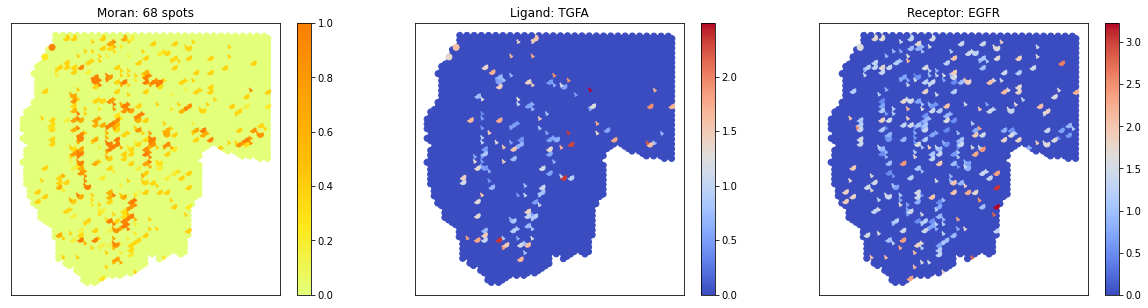
[38]:
# visualize 3 pairs in a pattern
pl.plot_pairs(A1, ['TGFA_EGFR','EGF_EGFR'], cmap='Wistia')

[41]:
# double check if the last column is cell type or not
A1.obsm['celltypes'] = A1.obs[A1.obs.columns[:-1]]
pl.chord_celltype(A1, pairs=['TGFA_EGFR','EGF_EGFR'], ncol=2, min_quantile=0.01)
# save='A1_EGF.svg'
[41]:
Note
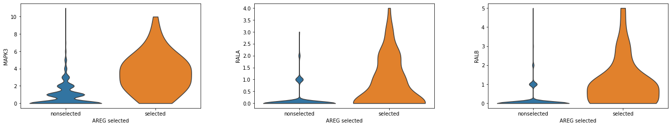
MAPK and RAL are reported upstream and downstream effectors of EGF, respectively. We examine if they express at the identified spots Please refer to our manuscript for more discussions.
[42]:
A1.obs['AREG_selected'] = np.where(A1.uns['selected_spots'].loc['AREG_EGFR'].values, 'selected','nonselected')
[43]:
import scanpy as sc
sc.pl.violin(A1, ['MAPK3','RALA', 'RALB'], 'AREG_selected', stripplot=False)
Cross-replicate consistency
Thanks to the multi-replicate setting, we could validate the consistency between biological / technical replicates
Global consistency
[29]:
I_df = pd.DataFrame(pd.Series(sample.uns['global_I'], index=sample.uns['global_res'].index) for sample in samples)
I_df = I_df.transpose()
I_df.columns = data
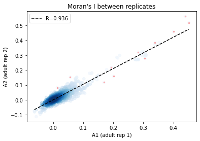
Extract the Global R from each replicate.
[30]:
from hilearn import *
_df = I_df.loc[:, ['A1', 'A2']].dropna()
corr_plot(_df.A1.values, _df.A2.values)
plt.xlabel('A1 (adult rep 1)')
plt.ylabel('A2 (adult rep 2)')
plt.title('Moran\'s I between replicates')
[30]:
Text(0.5, 1.0, "Moran's I between replicates")
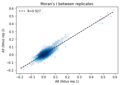
[31]:
_df = I_df.loc[:, ['A8', 'A9']].dropna()
corr_plot(_df.A8.values, _df.A9.values)
plt.xlabel('A8 (fetus rep 1)')
plt.ylabel('A9 (fetus rep 2)')
plt.title('Moran\'s I between replicates')
[31]:
Text(0.5, 1.0, "Moran's I between replicates")
[32]:
_df = I_df.loc[:, ['A2', 'A9']].dropna()
corr_plot(_df.A2.values, _df.A9.values)
plt.xlabel('A2 (adult rep 1)')
plt.ylabel('A9 (fetus rep 2)')
plt.title('Moran\'s I between non-biological replicates')
[32]:
Text(0.5, 1.0, "Moran's I between non-biological replicates")
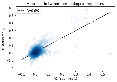
From the above results, Global R is consistent between replicates.
Local consistency & selected cell type consistency
We can also assess the local selection consistency by comparing the cell type compositions of selected spots
[33]:
fetus_celltypes = A3.obs.columns
PLG_df = pd.DataFrame(fetus_celltypes, index=fetus_celltypes)
PLG_F2RL1 is sparsely detected in fetus samples, it will be interesting to see whether such selections are consistent.
[34]:
pair='PLG_F2RL1'
for d,sample in zip(data,samples):
sample.celltype = locals()['{}'.format(d)].obs
if pair in sample.uns['local_z_p'].index:
ct=sample.celltype[sample.uns['local_z_p'].loc[pair].values<0.1].sum(0).sort_values(ascending=False)
ct=ct[ct>0]
PLG_df['{}'.format(d)]=ct
else:
PLG_df['{}'.format(d)] = 0
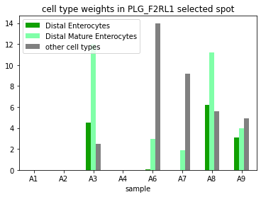
Group spot weights by selecte cell type vs other cell types
[35]:
PLG_df.pop(0)
other=PLG_df.loc[~PLG_df.index.isin(['Distal Enterocytes','Distal Mature Enterocytes'])].sum(0)
df =pd.concat((PLG_df.loc[PLG_df.index.isin(['Distal Enterocytes','Distal Mature Enterocytes'])],
pd.DataFrame(other, columns=['other cell types']).transpose()))
df = df.transpose()
df['sample']=df.index
PLG_F2RL1 is enriched in Enterocytes in 12-PCW colons, but not found in 19-PCW and adult samples. The two 12-PCW TI samples also have consistent PLG_F2RL1 enrichment, but the signaling celltypes are different from colon samples.
[36]:
plt.figure()
ax=df.sort_index().plot(x='sample',
kind='bar',
stacked=False,
title='cell type weights in PLG_F2RL1 selected spot',
color={'Distal Mature Enterocytes': [0.5 , 1. , 0.65808859, 1. ],
'Distal Enterocytes': [0.06331813, 0.62857143, 0. , 1. ],
# 'neuron':[0.99848342, 0.875 , 0.99522066, 1. ],
'other cell types': 'grey'})
ax.set_xticklabels(df.sort_index().index, rotation=0)
[36]:
[Text(0, 0, 'A1'),
Text(1, 0, 'A2'),
Text(2, 0, 'A3'),
Text(3, 0, 'A4'),
Text(4, 0, 'A6'),
Text(5, 0, 'A7'),
Text(6, 0, 'A8'),
Text(7, 0, 'A9')]
<Figure size 432x288 with 0 Axes>